.ipynb .pdf

repository open issue

Binder Live Code

Contents

Chapter 01: Log-Linear Model

1. Introduction

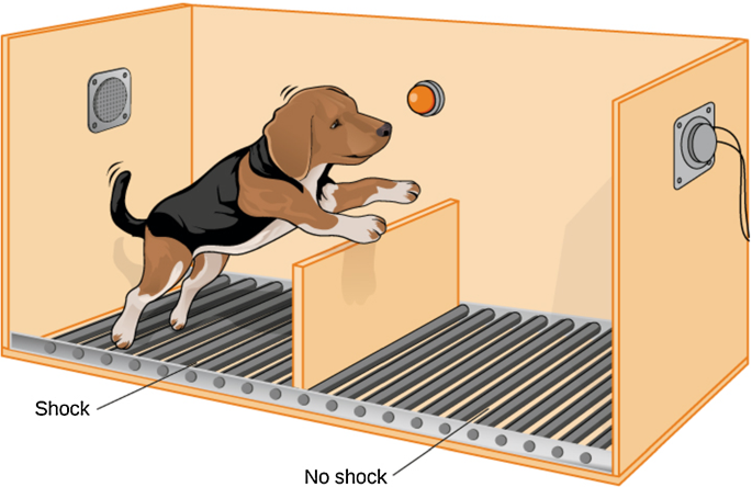
Solomon and Wynne conducted an experiment on Dogs in 1953 . They wanted to understand, whether Dogs can learn from mistakes, so to speak. Specifically, they were interested in avoidance-learning. That is, when Dogs are given trauma-inducing shocks, will they learn to avoid shocks in future?

We can state the objectives of the expeirment, according to our understanding, in more general terms as follows:

1. Can the Dogs learn?

2. Can they retain & recollect what they learnt?

The experimental setup, to drive the objectives, holds a dog in a closed compartment with steel flooring, open on one side with a small barrier for dog to jump over to the other side. A high-voltage electric shock is discharged into the steel floor intermittently to stimulate the dog. The dog is then left with an option to either get the shock for that trial or jump over the barrier to the other side & save himself. Several dogs were recruited in the experiment.

The following picture (source) is an illustration of the setup.



More details of the experiment can be found here.

In this chapter, we will analyze the experimental data using Bayesian Analysis, and the inference will be carried out in Pyro. The organization of the notebook is inspired from Bayesian Workflow by Prof. Andrew Gelman et al. Another piece of work in that direction is from Betancourt et al here. However, the current analysis is a WIP and far from perfect.

An almost always first step in Bayesian Analysis is to elicit a plausible generative model, that would have likely generated the observed data. In this case, consider the model suggested/implemented in WinBUGs Vol1.

We want to model the relationship between avoidance-in-future and past-traumatic-experiences. The following log-linear model is a starting point:

\(\pi_j = A^{xj} B^{j-xj} \)

where :

• \(\pi_j\) is the probability of a dog getting shocked at trial \(j\).

• \(x_j\) is number of successful avoidances of shock prior to trial \(j\).

• \(j-x_j\) is number of shocks experienced prior to trial \(j\).

• A & B, both are unknown and treated as random variables.

However, the model is only partially complete. In a Bayesian setting, we need to elicit our prior beliefs about the unknowns. Consequently, we need to give priors to \(A\) and \(B\), which we do shortly. Before that, we need some boiler plate code, mostly imports. Note that, all the code (functions) are glued in the base class. If one is interested, they can always browse the code repo to get better understanding.

import torch
import pyro
import pandas as pd
import itertools
from collections import defaultdict
import matplotlib.pyplot as plt
import pyro.distributions as dist
import seaborn as sns
import plotly
import plotly.express as px
import plotly.figure_factory as ff
from chapter01 import base
import numpy as np

pyro.set_rng_seed(1)

plt.style.use('default')

%matplotlib inline
%load_ext autoreload

Data

The data contains experiments over 30 dogs and each dog is subjected to 25 trials.

The plot that follows highlights Dogs data in dictionary format, averaged over dog population for each trial, i.e., \(y_j = \frac{1}{30}\sum{y_{ij}}\) where \(y_{ij}\) is the i-th Dog’s response at the j-th trial.

dogs_data = base.load_data()
base.plot_original_y(1-np.mean(dogs_data["Y"], axis=0), ylabel='Probability of shock at trial j')

Its apparent from experimental data that more than half the dog population learns to avoid shocks in trials as few as 5, and also that the learning doesn’t significantly rise with increased number of trials.

Preprocessing

Next, we need to transform raw data to obtain:

• x_avoidance : number of shock avoidances before current trial.

• x_shocked : number of shocks before current trial.

• y : status ‘shocked (y=1) or avoided(y=0)’ at current trial.

Here pystan format data (python dictionary) is passed to the function above, in order to preprocess it to the tensor format required for pyro sampling.

x_avoidance, x_shocked, y = base.transform_data(**dogs_data)
print("x_avoidance: %s, x_shocked: %s, y: %s"%(x_avoidance.shape, x_shocked.shape, y.shape))
print("\nSample x_avoidance: %s \n\nSample x_shocked: %s"%(x_avoidance[1], x_shocked[1]))

base.plot_original_y(x_avoidance.numpy(), ylabel='Cumulative Avoidances')
base.plot_original_y(x_shocked.numpy(), ylabel='Cumulative Shocked Trials')

x_avoidance: torch.Size([30, 25]), x_shocked: torch.Size([30, 25]), y: torch.Size([30, 25])

Sample x_avoidance: tensor([0., 0., 0., 0., 0., 0., 0., 0., 0., 1., 1., 1., 1., 1., 1., 1., 1., 1.,
        1., 1., 1., 1., 2., 2., 3.]) 

Sample x_shocked: tensor([ 0.,  1.,  2.,  3.,  4.,  5.,  6.,  7.,  8.,  8.,  9., 10., 11., 12.,
        13., 14., 15., 16., 17., 18., 19., 20., 20., 21., 21.])

The original data is not revealing much; looking at the cumulative avoidances and shocks, we see that some dogs never learn (example: Dog 1-4), and some dogs learn and retain the learning behaviour (example: Dog 25-30).

2. Model Specification

---

The sampling distribution of the generative model, as indicated earlier is:

\(y_{ij} \sim Bern(\pi_{ij})\)
\(\log(\pi_{ij}) = \alpha x_{ij} + \beta\ ({j-x_{ij}})\)

Here, \(y_{ij}=1\) if the \(i^{th}\) dog fails to avoid a shock at the \(j^{th}\) trial, and is 0 if it avoids.

The above expression is used as a generalised linear model with log-link function in WinBugs implementation

BUGS model

In WinBUGs, the model is:

\(\log(\pi_{j}) = \alpha x_{j} + \beta({j-x_{j}})\)

Here

• \(\log\pi_j\) is log probability of a dog getting shocked at trial \(j\).

• \(x_j\) is the number of successful avoidances of shock prior to trial \(j\).

• \(j-x_j\) is the number of shocks experienced prior to trial \(j\).

• \(\alpha\) & \(\beta\) are the unknowns.

Following code block is from original BUGS volume:

    {
        for (i in 1 : Dogs) {
        xa[i, 1] <- 0; xs[i, 1] <- 0 p[i, 1] <- 0
        for (j in 2 : Trials) {
        xa[i, j] <- sum(Y[i, 1 : j - 1])
        xs[i, j] <- j - 1 - xa[i, j]
        log(p[i, j]) <- alpha * xa[i, j] + beta * xs[i, j]
        y[i, j] <- 1 - Y[i, j]
        y[i, j] ~ dbern(p[i, j])
       }
    }
    alpha ~ dnorm(0, 0.00001)I(, -0.00001)
    beta ~ dnorm(0, 0.00001)I(, -0.00001)
    A <- exp(alpha)
    B <- exp(beta)
    }

---

Stan model

The same model in PyStan is implemented as follows:

{
    alpha ~ normal(0.0, 316.2);
    beta  ~ normal(0.0, 316.2);
    for(dog in 1:Ndogs)
        for (trial in 2:Ntrials)  
            y[dog, trial] ~ bernoulli(exp(alpha * xa[dog, trial] + beta * xs[dog, trial]));
      
}  

In the orginal WinBUGS reference, \(\alpha, \beta\) are given truncated Normal priors, but not in Stan. Note that \(\pi_{ij} > 1\) when \(\alpha, \beta > 0\). Thefore, we have to restrict \(\alpha, \beta \le 0\)

Consequently, we elicit half-normal priors for \(\alpha,\beta\) with zero mean and large variance (flat) to complete the specification. Also notice that, the above model is in a more familiar form (Generalized Linear Model or Log-Linear Model). For convenience, we can define \(X_{a}\equiv x_{ij},\ X_{s}\equiv j-x_{ij} \)

The complete model is:

\(y_{ij} \sim Bern(\pi_{ij})\)
\(\log(\pi_{ij}) = \alpha X_{a} + \beta X_{s}\) or \(\pi_{ij} = e^{(\alpha X_{a} + \beta X_{s})}\)
\(\alpha \sim N(0., 316.)I(\alpha <0)\)
\(\beta \sim N(0., 316.)I(\beta <0)\)

But it is easier to constrain R.Vs on the positive real line. So, we simply absorb the negative sign inside the model. Finally, we have these models, with Half-normal and Uniform priors s.t \(\alpha, \beta > 0\). They are:

Model A.
\(y_{ij} \sim Bern(\pi_{ij})\)
\(\pi_{ij} = e^{(-(\alpha X_{a} + \beta X_{s}))}\)

\(\alpha \sim N(0., 316.)\ I(\alpha>0)\)
\(\beta \sim N(0., 316.)\ I(\beta>0)\)

Model B.
\(y_{ij} \sim Bern(\pi_{ij})\)
\(\pi_{ij} = e^{(-(\alpha X_{a} + \beta X_{s}))}\)

\(\alpha \sim U(0, 10.)\)
\(\beta \sim U(0, 10.)\)

Model implementation

The above models are defined in base.DogsModel

DogsModel= base.DogsModel

DogsModel

<function chapter01.base.DogsModel(x_avoidance, x_shocked, y, alpha_prior=None, beta_prior=None, activation='exp')>

Let us also draw few samples from the prior, and look at the distribution

num_samples = 1100 

alpha_prior_a, beta_prior_a= base.init_priors({"default":dist.HalfNormal(316.)})# Pass priors for model A
prior_samples_a = base.get_prior_samples(alpha_prior_a, beta_prior_a, num_samples=num_samples)

alpha_prior_b, beta_prior_b= base.init_priors({"default":dist.Uniform(0.001, 10)})# Pass uniform priors for model B
prior_samples_b = base.get_prior_samples(alpha_prior_b, beta_prior_b, num_samples=num_samples)

Sampled output of prior values for \(\alpha\) & \(\beta\) are stored in prior_samples above, and are plotted on a KDE plot as follows:

base.plot_prior_distributions(model_halfnormal_a= prior_samples_a, model_uniform_b= prior_samples_b)

For model 'model_halfnormal_a' Prior alpha Q(0.5) :206.15262603759766 | Prior beta Q(0.5) :206.13883209228516

For model 'model_uniform_b' Prior alpha Q(0.5) :5.179362535476685 | Prior beta Q(0.5) :5.287136554718018

3. Prior predictive checking

Prior predictive checking (PiPC)

original_plus_simulated_prior_data = base.simulate_observations_given_prior_posterior_pairs(dogs_data["Y"], num_dogs=30, num_trials=24, 
                                                                                            activation_type= "exp", model_halfnormal_a= prior_samples_a, 
                                                                                            model_uniform_b= prior_samples_b)

___________

For model 'model_halfnormal_a' prior
total samples count: 1100  sample example:  [(208.98727416992188, 84.3480224609375), (19.490013122558594, 196.33627319335938)]
Total execution time: 75.1559419631958

Number of datasets/prior pairs generated: 1100
Shape of data simulated from prior for model 'model_halfnormal_a' : (25,)
___________

For model 'model_uniform_b' prior
total samples count: 1100  sample example:  [(5.8912200927734375, 0.18410980701446533), (7.265109539031982, 2.5937607288360596)]
Total execution time: 74.87336492538452

Number of datasets/prior pairs generated: 1100
Shape of data simulated from prior for model 'model_uniform_b' : (25,)
Respective shape of original data: (25,) and concatenated arrays of data simulated for different priors/posteriors: (3, 25)

_______________________________________________________
______________________________________________________________________
Here 'Dog_1' corresponds to observations simulated from prior of 'model_halfnormal_a', 'Dog_2' corresponds to observations simulated from prior of 'model_uniform_b' & 'Dog_3' corresponds to 'Original data'.

We notice something very strange. We thought the priors on \(\alpha, \beta\) are flat, which is true, but naively we assumed they will turn out to be non-informative as well.

But they are not non-informative. In fact, they are extremely informative for \(\pi_{ij}\), since a priori, it has a right skewed distribution, with mode at 0. As a result, a priori, we think that, Dogs getting shocked has a very low chance.

Lets investigate it little more formally. Say, we observed \(X_a=1, X_s=0\), and also consider uniform priors \(U(0,b), b>0\) for both \(\alpha,\beta\).

Then, \(\pi = e^{-\alpha}\) with \(\alpha \sim U(0,b)\). We can calculate the prior expected value analytically, as follows:

\[\begin{equation} E_{pr}[\hat{y}] = \frac{1}{b}\int_{0}^{b} e^{-\alpha} = (1-e^{-b})/b \end{equation} \]

with \(\lim_{b \to 0} E_{pr}[\hat{y}] = 1 \) and \(\lim_{b \to \infty} E_{pr}[\hat{y}] = 0 \) implying that, for supposedly a non-informative prior, we have strong prior belief that Dogs will avoid shocks, with certainity.

Let us generalize the setting further. Suppose, we are at the n-th trial. Let \(x_a, \ x_s\) be the avoidances and shocks upto this trial, respectively. Then,

\[\begin{equation} E_{pr}[\hat{y}] = \frac{1}{b^2}\int_{0}^{b} e^{-\alpha x_a} \int_{0}^{b} e^{-\beta x_s} = \frac{1}{b^2 x_a x_s}(1-e^{-bx_a})(1-e^{-bx_s}) \end{equation} \]

Notice that, as the number of trials \(n = x_a+x_s+1\) increases, the expected values decreases to 0 at rate \(O(1/b^2n)\). Thefore, eventually, Dogs learn-to-avoid with certainty, is the a priori behaviour.

4. Posterior Estimation

In the Bayesian setting, inference is drawn from the posterior. Here, posterior implies the updated beliefs about the random variables, in the wake of given evidences (data). Formally,

\(Posterior = \frac {Likelihood x Prior}{Probability \ of Evidence}\)

In our case, \(\alpha,\beta\) are the parameters (actually random variables) & \(y\) is the evidence; According to the Bayes rule, Posterior \(P(\alpha,\beta | y)\) is given as:

\(P\ (\alpha,\beta | y) = \frac {P(y | \alpha,\beta) \pi(\alpha,\beta)}{P(y)}\)

Now our interest is in estimating the posterior summaries of the parameters \(\alpha, \beta\). For example, we can look at the posterior of mean of \(\alpha\), denoted as \(E(\alpha)\). However, in order to the get the posterior quanitities, either we need to compute the integrals or approximate the integrals via Markov Chain Monte Carlo.

The latter can be easily accomplished in Pyro by using the NUTS sampler – NUTS is a specific sampler designed to draw samples efficiently from the posterior using Hamiltonian Monte Carlo dynamics.

The following code snippet takes a pyro model object with – posterior specification, input data, some configuration parameters such as a number of chains and number of samples per chain. It then launches a NUTS sampler and produces MCMC samples in a python dictionary format.

# DogsModel_A alpha, beta ~ HalfNormal(316.) & activation "exp"

hmc_sample_chains_a, hmc_chain_diagnostics_a = base.get_hmc_n_chains(DogsModel, x_avoidance, x_shocked, y, num_chains=4, 
                                                                     sample_count = 900, alpha_prior= dist.HalfNormal(316.), 
                                                                     beta_prior= dist.HalfNormal(316.), activation= "exp")

Sample: 100%|██████████| 11000/11000 [00:51, 213.95it/s, step size=9.31e-01, acc. prob=0.909]
Sample: 100%|██████████| 11000/11000 [00:42, 257.06it/s, step size=9.47e-01, acc. prob=0.881]
Sample: 100%|██████████| 11000/11000 [00:53, 205.76it/s, step size=7.71e-01, acc. prob=0.915]
Sample: 100%|██████████| 11000/11000 [00:53, 204.40it/s, step size=8.01e-01, acc. prob=0.928]

Total time:  202.18049597740173

# DogsModel_B alpha, beta ~ Uniform(0., 10.0) & activation "exp"

hmc_sample_chains_b, hmc_chain_diagnostics_b = base.get_hmc_n_chains(DogsModel, x_avoidance, x_shocked, y, num_chains=4, sample_count = 900, 
                         alpha_prior= dist.Uniform(0., 10.0), beta_prior= dist.Uniform(0., 10.0), activation= "exp")

Sample: 100%|██████████| 11000/11000 [00:50, 218.81it/s, step size=7.54e-01, acc. prob=0.927]
Sample: 100%|██████████| 11000/11000 [00:48, 224.73it/s, step size=7.89e-01, acc. prob=0.927]
Sample: 100%|██████████| 11000/11000 [00:49, 221.43it/s, step size=8.69e-01, acc. prob=0.916]
Sample: 100%|██████████| 11000/11000 [00:40, 273.05it/s, step size=9.71e-01, acc. prob=0.897]

Total time:  189.7234182357788

hmc_sample_chains holds sampled MCMC values as {"Chain_0": {alpha [-0.20020795, -0.1829252, -0.18054989 . .,], "beta": {}. .,}, "Chain_1": {alpha [-0.20020795, -0.1829252, -0.18054989 . .,], "beta": {}. .,}. .}

5. MCMC Diagnostics

Diagnosing the computational approximation

Just like any numerical technique, no matter how good the theory is or how robust the implementation is, it is always a good idea to check if indeed the samples drawn are reasonable. In the ideal situation, we expect the samples drawn by the sampler to be independant, and identically distributed (i.i.d) as the posterior distribution. In practice, this is far from true as MCMC itself is an approximate technique and a lot can go wrong. In particular, chains may not have converged or samples are very correlated. We can divide diagnosis into three sections.

• Burn-in: What is the effect of initialization? By visually inspecting the chains, we can notice the transient behaviour. We can drop the first “n” number of samples from the chain.

• Thinning: What is the intra chain correlation? We can use ACF (Auto-correlation function) to inspect it. A rule of thumb is, thin the chains such that, the ACF drops to \(1/10^{th}\). Here, ACF drops to less than 0.1 at lag 5, then we retain only every \(5^{th}\) sample in the chain.

• Mixing: Visually, all the chains, when plotted, should be indistinguishable from each other. At a very broad level, the means of the chains and variances shall be close. These are the two central moments we can track easily and turn them into Gelman-Rubin statistic. Other summmary statistics can be tracked, of course.

We can use both visual and more formal statistical techniques to inspect the quality of the fit (not the model fit to the data, but how well the approximation is, having accepted the model class for the data at hand) by treating chains as time-series data, and that we can run several chains in parallel. We precisely do that next.

Following snippet allows plotting Parameter vs. Chain matrix and optionally saving the dataframe.

Model-A Summaries

# Unpruned sample chains for model A with HalfNormal prior

beta_chain_matrix_df_A = pd.DataFrame(hmc_sample_chains_a)

base.save_parameter_chain_dataframe(beta_chain_matrix_df_A, "data/dogs_parameter_chain_matrix_1A.csv")

Saved at 'data/dogs_parameter_chain_matrix_1A.csv'

A.1 Visual summary

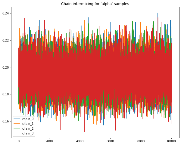
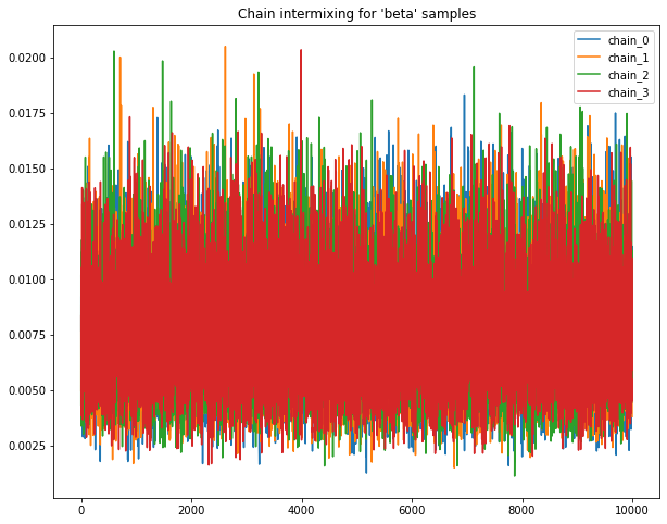
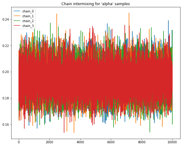
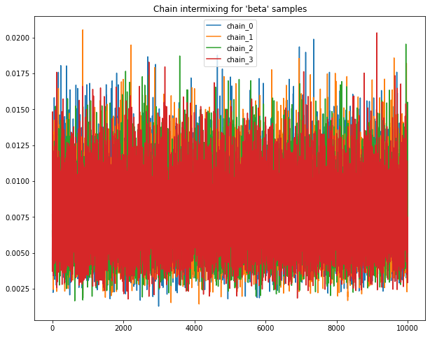
A.1.1 Intermixing chains

Sample chains mixing for HalfNormal priors.

Following plots chains of samples for alpha & beta parameters for model_HalfNormal_a

base.plot_chains(beta_chain_matrix_df_A)

for chain, samples in hmc_sample_chains_a.items():
    print("____\nFor 'model_HalfNormal_a' %s"%chain)    
    samples= dict(map(lambda param: (param, torch.tensor(samples.get(param))), samples.keys()))# np array to tensors
    print(chain, "Sample count: ", len(samples["alpha"]))
    print("Alpha Q(0.5) :%s | Beta Q(0.5) :%s"%(torch.quantile(samples["alpha"], 0.5), torch.quantile(samples["beta"], 0.5)))

____
For 'model_HalfNormal_a' chain_0
chain_0 Sample count:  10000
Alpha Q(0.5) :tensor(0.1936) | Beta Q(0.5) :tensor(0.0073)
____
For 'model_HalfNormal_a' chain_1
chain_1 Sample count:  10000
Alpha Q(0.5) :tensor(0.1938) | Beta Q(0.5) :tensor(0.0073)
____
For 'model_HalfNormal_a' chain_2
chain_2 Sample count:  10000
Alpha Q(0.5) :tensor(0.1937) | Beta Q(0.5) :tensor(0.0073)
____
For 'model_HalfNormal_a' chain_3
chain_3 Sample count:  10000
Alpha Q(0.5) :tensor(0.1935) | Beta Q(0.5) :tensor(0.0073)

A.2 Quantitative summary

A.2.1 ACF plots

Auto-correlation plots for sample chains with HalfNormal priors

base.autocorrelation_plots(beta_chain_matrix_df_A)

• For alpha, thining factor for chain_0 is 3, chain_1 is 3, chain_2 is 3, chain_3 is 3

• For beta, thinin factor for chain_0 is 3, chain_1 is 3, chain_2 is 3, chain_3 is 3

Pruning chains from model with HalfNormal priors

thining_dict_a = {"chain_0": {"alpha":3, "beta":3}, "chain_1": {"alpha":3, "beta":3}, 
                "chain_2": {"alpha":3, "beta":3}, "chain_3": {"alpha":3, "beta":3}}

pruned_hmc_sample_chains_a = base.prune_hmc_samples(hmc_sample_chains_a, thining_dict_a)

-------------------------
Original sample counts for 'chain_0' parameters: {'alpha': (10000,), 'beta': (10000,)}

Thining factors for 'chain_0' parameters: {'alpha': 3, 'beta': 3} 
Post thining sample counts for 'chain_0' parameters: {'alpha': (3333,), 'beta': (3333,)}


-------------------------
Original sample counts for 'chain_1' parameters: {'alpha': (10000,), 'beta': (10000,)}

Thining factors for 'chain_1' parameters: {'alpha': 3, 'beta': 3} 
Post thining sample counts for 'chain_1' parameters: {'alpha': (3333,), 'beta': (3333,)}


-------------------------
Original sample counts for 'chain_2' parameters: {'alpha': (10000,), 'beta': (10000,)}

Thining factors for 'chain_2' parameters: {'alpha': 3, 'beta': 3} 
Post thining sample counts for 'chain_2' parameters: {'alpha': (3333,), 'beta': (3333,)}


-------------------------
Original sample counts for 'chain_3' parameters: {'alpha': (10000,), 'beta': (10000,)}

Thining factors for 'chain_3' parameters: {'alpha': 3, 'beta': 3} 
Post thining sample counts for 'chain_3' parameters: {'alpha': (3333,), 'beta': (3333,)}

A.2.2 G-R statistic

Gelman-Rubin statistic for chains with HalfNormal priors

grubin_values_a = base.gelman_rubin_stats(pruned_hmc_sample_chains_a)

Gelmen-rubin for 'param' alpha all chains is: 0.9997

Gelmen-rubin for 'param' beta all chains is: 0.9998

A.3 Descriptive summary

Following outputs the summary of required statistics such as "mean", "std", "Q(0.25)", "Q(0.50)", "Q(0.75)", select names of statistic metric from given list to view values.

A.3.1 Summary Table 1

Tabulated Summary for model chains with HalfNormal priors

#chain results Pruned after ACF plots

beta_chain_matrix_df_A = pd.DataFrame(pruned_hmc_sample_chains_a)

base.summary(beta_chain_matrix_df_A)

Select any value

We can also report the 5-point Summary Statistics (mean, Q1-Q4, Std, ) as tabular data per chain and save the dataframe

fit_df_A = pd.DataFrame()
for chain, values in pruned_hmc_sample_chains_a.items():
    param_df = pd.DataFrame(values)
    param_df["chain"]= chain
    fit_df_A= pd.concat([fit_df_A, param_df], axis=0)

base.save_parameter_chain_dataframe(fit_df_A, "data/dogs_classification_hmc_samples_1A.csv")

Saved at 'data/dogs_classification_hmc_samples_1A.csv'

Use following button to upload:

• "data/dogs_classification_hmc_samples_1A.csv" as 'fit_df_A'

# Use following to load data once the results from pyro sampling operation are saved offline
load_button= base.build_upload_button()

# Use following to load data once the results from pyro sampling operation are saved offline

if load_button.value:
    fit_df_A = base.load_parameter_chain_dataframe(load_button)#Load "data/dogs_classification_hmc_samples_1A.csv"

A.3.2 Summary Table 2

5-point Summary Statistics for model chains with HalfNormal priors

Following outputs the similar summary of required statistics such as "mean", "std", "Q(0.25)", "Q(0.50)", "Q(0.75)", but in a slightly different format, given a list of statistic names

base.summary(fit_df_A, layout =2)

Select any value

Following plots sampled parameters values as Boxplots with M parameters side by side on x axis for each of the N chains.

Pass the list of M parameters and list of N chains, with plot_interactive as True or False to choose between Plotly or Seaborn

A.4 Additional plots

A.4.1 Boxplots

Boxplot for model chains with HalfNormal priors

parameters= ["alpha", "beta"]# All parameters for given model
chains= fit_df_A["chain"].unique()# Number of chains sampled for given model

# Use plot_interactive=False for Normal seaborn plots offline

base.plot_parameters_for_n_chains(fit_df_A, chains=['chain_0', 'chain_1', 'chain_2', 'chain_3'], parameters=parameters, plot_interactive=True)

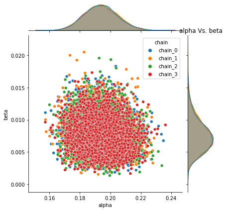
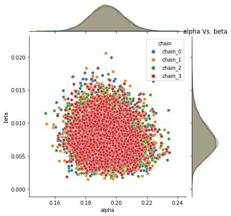
A.4.2 Joint distribution plots

Following plots the joint distribution of pair of each parameter sampled values for all chains with HalfNormal priors.

base.plot_joint_distribution(fit_df_A, parameters)

Pyro -- alpha Vs. beta

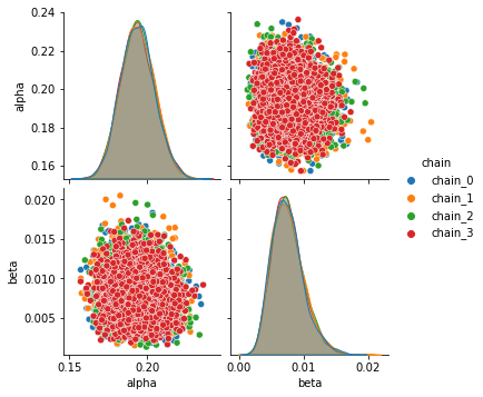
A.4.3 Pairplots

Following plots the Pairplot distribution of each parameter with every other parameter’s sampled values for all chains with HalfNormal priors

sns.pairplot(data=fit_df_A, hue= "chain");

Model-B Summaries

# Unpruned sample chains for model B with Uniform prior

beta_chain_matrix_df_B = pd.DataFrame(hmc_sample_chains_b)

base.save_parameter_chain_dataframe(beta_chain_matrix_df_B, "data/dogs_parameter_chain_matrix_1B.csv")

Saved at 'data/dogs_parameter_chain_matrix_1B.csv'

B.1 Visual summary

B.1.1 Intermixing chains

Sample chains mixing for Uniform priors.

Following plots chains of samples for alpha & beta parameters for model_Uniform_b

base.plot_chains(beta_chain_matrix_df_B)

for chain, samples in hmc_sample_chains_b.items():
    print("____\nFor 'model_Uniform_b' %s"%chain)    
    samples= dict(map(lambda param: (param, torch.tensor(samples.get(param))), samples.keys()))# np array to tensors
    print(chain, "Sample count: ", len(samples["alpha"]))
    print("Alpha Q(0.5) :%s | Beta Q(0.5) :%s"%(torch.quantile(samples["alpha"], 0.5), torch.quantile(samples["beta"], 0.5)))

____
For 'model_Uniform_b' chain_0
chain_0 Sample count:  10000
Alpha Q(0.5) :tensor(0.1938) | Beta Q(0.5) :tensor(0.0073)
____
For 'model_Uniform_b' chain_1
chain_1 Sample count:  10000
Alpha Q(0.5) :tensor(0.1935) | Beta Q(0.5) :tensor(0.0074)
____
For 'model_Uniform_b' chain_2
chain_2 Sample count:  10000
Alpha Q(0.5) :tensor(0.1934) | Beta Q(0.5) :tensor(0.0073)
____
For 'model_Uniform_b' chain_3
chain_3 Sample count:  10000
Alpha Q(0.5) :tensor(0.1936) | Beta Q(0.5) :tensor(0.0074)

B.2 Quantitative summary

B.2.1 ACF plots

Auto-correlation plots for sample chains with Uniform priors

base.autocorrelation_plots(beta_chain_matrix_df_B)

• For alpha, thining factor for chain_0 is 3, chain_1 is 3, chain_2 is 3, chain_3 is 3

• For beta, thinin factor for chain_0 is 3, chain_1 is 3, chain_2 is 3, chain_3 is 3

Pruning chains from model with Uniform priors

thining_dict_b = {"chain_0": {"alpha":3, "beta":3}, "chain_1": {"alpha":3, "beta":3}, 
                "chain_2": {"alpha":3, "beta":3}, "chain_3": {"alpha":3, "beta":3}}

pruned_hmc_sample_chains_b = base.prune_hmc_samples(hmc_sample_chains_b, thining_dict_b)

-------------------------
Original sample counts for 'chain_0' parameters: {'alpha': (10000,), 'beta': (10000,)}

Thining factors for 'chain_0' parameters: {'alpha': 3, 'beta': 3} 
Post thining sample counts for 'chain_0' parameters: {'alpha': (3333,), 'beta': (3333,)}


-------------------------
Original sample counts for 'chain_1' parameters: {'alpha': (10000,), 'beta': (10000,)}

Thining factors for 'chain_1' parameters: {'alpha': 3, 'beta': 3} 
Post thining sample counts for 'chain_1' parameters: {'alpha': (3333,), 'beta': (3333,)}


-------------------------
Original sample counts for 'chain_2' parameters: {'alpha': (10000,), 'beta': (10000,)}

Thining factors for 'chain_2' parameters: {'alpha': 3, 'beta': 3} 
Post thining sample counts for 'chain_2' parameters: {'alpha': (3333,), 'beta': (3333,)}


-------------------------
Original sample counts for 'chain_3' parameters: {'alpha': (10000,), 'beta': (10000,)}

Thining factors for 'chain_3' parameters: {'alpha': 3, 'beta': 3} 
Post thining sample counts for 'chain_3' parameters: {'alpha': (3333,), 'beta': (3333,)}

B.2.2 G-R statistic

Gelman-Rubin statistic for chains with Uniform priors

grubin_values_b = base.gelman_rubin_stats(pruned_hmc_sample_chains_b)

Gelmen-rubin for 'param' alpha all chains is: 0.9998

Gelmen-rubin for 'param' beta all chains is: 0.9997

B.3 Descriptive summary

Following outputs the summary of required statistics such as "mean", "std", "Q(0.25)", "Q(0.50)", "Q(0.75)", select names of statistic metric from given list to view values

B.3.1 Summary Table 1

Tabulated Summary for model chains with Uniform priors

#chain results Pruned after ACF plots

beta_chain_matrix_df_B = pd.DataFrame(pruned_hmc_sample_chains_b)

base.summary(beta_chain_matrix_df_B)

Select any value

We can also report the 5-point Summary Statistics (mean, Q1-Q4, Std, ) as tabular data per chain and save the dataframe

fit_df_B = pd.DataFrame()
for chain, values in pruned_hmc_sample_chains_b.items():
    param_df = pd.DataFrame(values)
    param_df["chain"]= chain
    fit_df_B= pd.concat([fit_df_B, param_df], axis=0)

base.save_parameter_chain_dataframe(fit_df_B, "data/dogs_classification_hmc_samples_1B.csv")

Saved at 'data/dogs_classification_hmc_samples_1B.csv'

Use following button to upload:

• "data/dogs_classification_hmc_samples_1B.csv" as 'fit_df_B'

# Use following to load data once the results from pyro sampling operation are saved offline
load_button= base.build_upload_button()

# Use following to load data once the results from pyro sampling operation are saved offline

if load_button.value:
    fit_df_B= base.load_parameter_chain_dataframe(load_button)#Load "data/dogs_classification_hmc_samples_1B.csv"
    

B.3.2 Summary Table 2

5-point Summary Statistics for model chains with Uniform priors

Following outputs the similar summary of required statistics such as "mean", "std", "Q(0.25)", "Q(0.50)", "Q(0.75)", but in a slightly different format, given a list of statistic names

base.summary(fit_df_B, layout =2)

Select any value

Following plots sampled parameters values as Boxplots with M parameters side by side on x axis for each of the N chains.

Pass the list of M parameters and list of N chains, with plot_interactive as True or False to choose between Plotly or Seaborn

B.4 Additional plots

B.4.1 Boxplots

Boxplot for model chains with Uniform priors

parameters= ["alpha", "beta"]# All parameters for given model
chains= fit_df_B["chain"].unique()# Number of chains sampled for given model

# Use plot_interactive=False for Normal seaborn plots offline

base.plot_parameters_for_n_chains(fit_df_B, chains=['chain_0', 'chain_1', 'chain_2', 'chain_3'], parameters=parameters, plot_interactive=True)